When I began this project, I found that my fellow academics had already developed several formal scales to measure how people felt about AI. By scale, I mean a set of survey items that were developed by experts to measure a psychological construct. A psychological construct is an abstract trait or state existing in the human mind. Constructs are difficult to measure. I could use a ruler to easily measure the distance between your eyes, but the thoughts that live behind them do not yield so easily.
Think of introversion as an example construct. Some individuals are more introverted; they like to stay home, avoid crowds and read books. Others are extroverted; they like to go out, seek company and make small talk. This introversion construct is a trait with two poles; each individual lies somewhere on a continuum from very extroverted to very introverted. A scale is the instrument to map individuals onto the continuum. A good scale uses survey items to score introverts high and extroverts low.
In our case, we are interested in attitudes toward artificial intelligence. An attitude is a construct that represents how one feels about something. Attitudes have a valence: positive/liking/approach on one side and negative/disliking/avoid on the other.
Putting it all together, here we will explore scales for AI attitudes. In other words, I asked Americans to take several expert-crafted surveys intended to measure positive versus negative feelings toward this rapidly developing technology, and here we will compare the results.
Using a scale of 1 to 5, where 1 means no benefit and 5 means many benefits, to what extent do you think artificial intelligence has benefits?
Using a scale of 1 to 5, where 1 means no risk and 5 means many risks, to what extent do you think there are risks in artificial intelligence?
Code
# The file ai-scales-2023-wide-correlates.csv contains responses from a US representative sample of 498 respondents.# Download the file from a public Open Science Framework repository at https://osf.io/download/xr6ku/responses =read_csv("data/ai-scales-2023-wide-correlates.csv")# Put the two Lobera variables into long formatlobera_long <- responses %>%select(lobera_2020_ai_risk, lobera_2020_ai_benes) %>%pivot_longer(cols =everything(),names_to ="item",values_to ="response" ) %>%filter(!is.na(response)) %>%mutate(item =recode( item,lobera_2020_ai_risk ="Lobera AI Risk",lobera_2020_ai_benes ="Lobera AI Benefits" ),response =as.numeric(response) )# Summary statistics for annotationlobera_stats <- lobera_long %>%group_by(item) %>%summarize(mean =mean(response),sd =sd(response),N =n(),se = sd /sqrt(N),ci_low = mean -qt(.975, df = N -1) * se,ci_high = mean +qt(.975, df = N -1) * se,.groups ="drop" ) %>%mutate(label =paste0("Mean = ", round(mean, 2),"\nSD = ", round(sd, 2),"\nN = ", N,"\nSE = ", round(se, 2),"\n95% CI [", round(ci_low, 2), ", ", round(ci_high, 2), "]" ),x =2.4,y =Inf )book_source_caption =paste0("Source: Thinking Machines, Pondering Humans by Dr. Jason Jeffrey Jones")# Plotggplot(lobera_long, aes(x = response)) +geom_bar(width =0.8) +facet_wrap(~ item, nrow =1) +geom_text(data = lobera_stats,aes(x = x, y = y, label = label),inherit.aes =FALSE,hjust ="right",vjust =1.1,size =3.25 ) +scale_x_continuous(breaks =1:5,minor_breaks =NULL ) +coord_cartesian(xlim =c(0.5, 5.5)) +labs(x ="Response",y ="Count",title ="Distributions of Lobera AI Benefits and AI Risk Responses",caption = book_source_caption ) +theme(plot.caption =element_text(size=10, color ="#666666"))
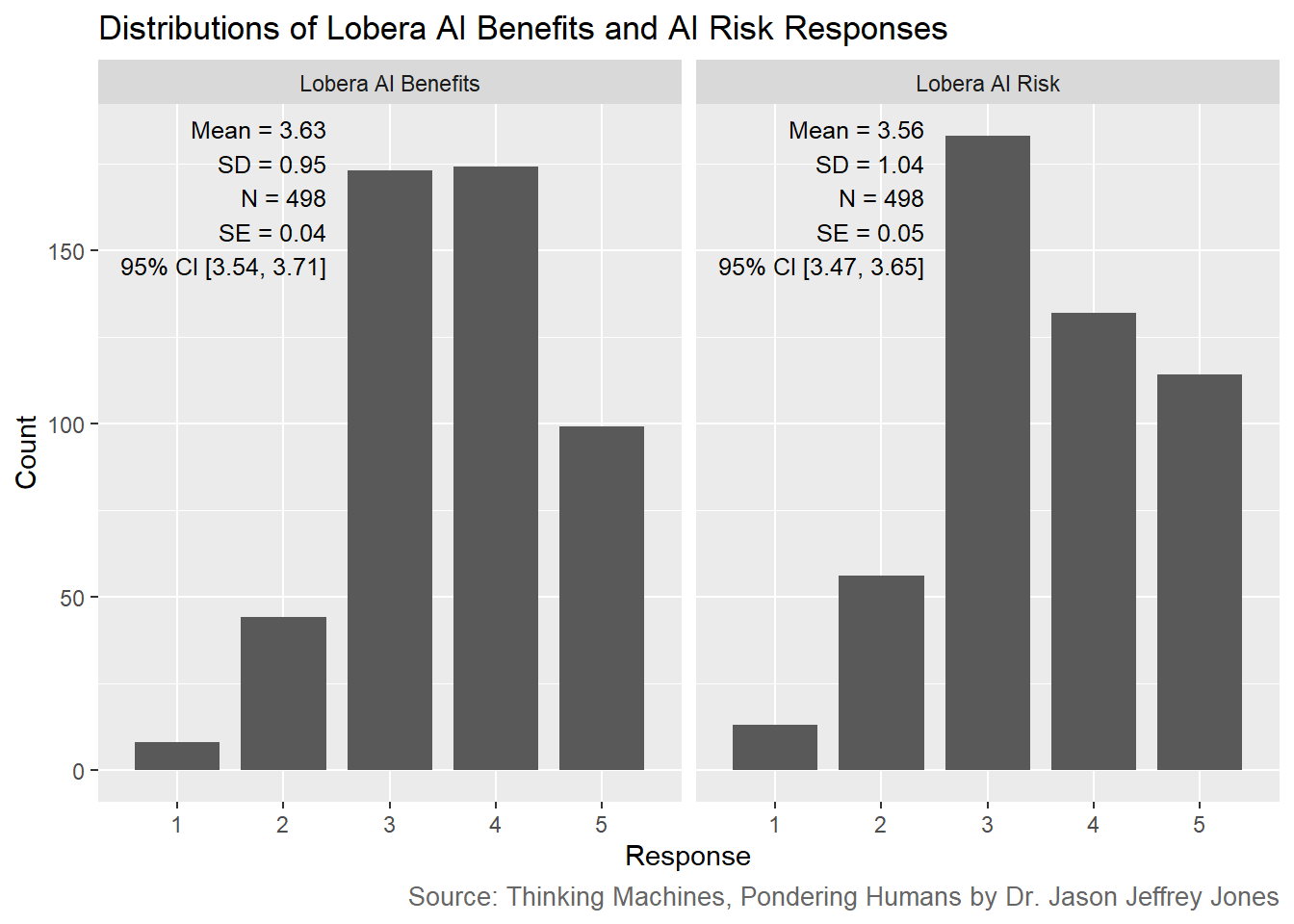
Figure 6.1: Histograms and descriptive statistics for Lobera AI attitude items.
Look at the very short bars for 1 responses in both histograms. These short bars tell us that almost no Americans saw AI as having no benefits or no risks.
An interesting question is whether perceived benefit and perceived risk were opposites, or whether the same respondents tended to see AI as both beneficial and risky.
We can answer that question by looking at responses from the same individuals and evaluating the correlation. A positive correlation would indicate that respondents saw AI as powerful and transformative: simultaneously risky and beneficial. A negative correlation tells a different story: respondents split themselves into groups by rating one higher than the other. In other words, one group saw more AI risk than benefits and (presumably) would recommend it be avoided. The other group saw high benefits with low risks and (presumably) would recommend it be pursued.
Before you look at the heatmap and correlation below, ask yourself what you predict.
Code
lobera_pair <- responses %>%transmute(ai_risk =as.numeric(lobera_2020_ai_risk),ai_benefits =as.numeric(lobera_2020_ai_benes) ) %>%filter(!is.na(ai_risk), !is.na(ai_benefits))lobera_heatmap <- lobera_pair %>%count(ai_benefits, ai_risk, name ="n") %>%complete(ai_benefits =1:5,ai_risk =1:5,fill =list(n =0) ) %>%mutate(pct = n /sum(n),label =paste0(n, "\n", percent(pct, accuracy =0.1)) )ggplot(lobera_heatmap, aes(x = ai_risk, y = ai_benefits, fill = n)) +geom_tile(color ="white") +geom_text(aes(label = label), size =3.25) +scale_fill_gradient(low ="grey95",high ="steelblue",trans ="sqrt",name ="Count" ) +scale_x_continuous(breaks =1:5) +scale_y_continuous(breaks =1:5) +coord_equal() +labs(x ="Perceived AI risks\n1 = no risks, 5 = many risks",y ="Perceived AI benefits\n1 = no benefits, 5 = many benefits",title ="Was AI Seen as Beneficial, Risky, or Both?",caption = book_source_caption ) +theme_minimal() +theme(plot.caption =element_text(size =10, color ="#666666") )
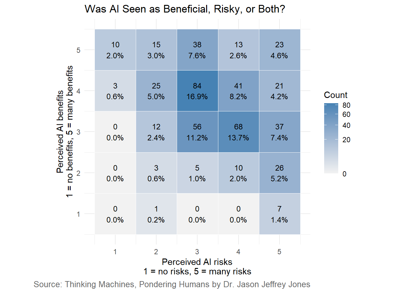
Figure 6.2: Joint distribution of perceived AI benefits and perceived AI risks.
Figure 6.2 and the modest negative correlation of -0.31 give an answer. Respondents tended to see more weight on one side or the other (risks versus benefits). But it is not the case that we see two well-defined blocks of risk-blind optimists versus benefit-blind pessimists. Most Americans occupied a mushy middle - rating both risk and benefit as three or four out of five.
6.1.1 Attitude Towards Artificial Intelligence (ATAI scale)
The Lobera items gave us a simple starting point: one question about AI benefits and one question about AI risks. Next, we move to the Attitude Towards Artificial Intelligence (ATAI) scale. (Great branding!) Developed by Sindermann and colleagues (2021), the ATAI comprises five items addressing fear, trust, existential risk, human benefit, and job loss. (Item wording appears in Section 6.2.1.)
Let’s examine Americans’ agreement with each of the five items.
Code
# Select columns and pivot.ataiResponses <- responses %>%select(starts_with("sinder_")) %>%pivot_longer(cols =everything(),names_to ="Item",names_prefix ="sinder_",values_to ="Response" ) %>%mutate(Item =recode( Item,"fear_ai"="Fear AI","trust_ai"="Trust AI","destroy_humankind"="Destroy Humankind","benefit_humankind"="Benefit Humankind","job_losses"="Cause Job Losses" ) )# Summary figureataiResponses %>%group_by(Item) %>%summarise(Mean_Response =mean(Response, na.rm =TRUE),sd =sd(Response, na.rm =TRUE),n =sum(!is.na(Response)),se = sd /sqrt(n),error_low = Mean_Response - se,error_high = Mean_Response + se ) %>%ggplot(aes(x =reorder(Item, Mean_Response), y = Mean_Response, color = Item, fill = Item)) +# Add green and red shading to demarcate agree vs disagree.annotate(geom="rect", xmin=-Inf, xmax=Inf, ymin=0.0, ymax=Inf, fill="green", alpha=0.1) +annotate(geom="rect", xmin=-Inf, xmax=Inf, ymin=-Inf, ymax=0.0, fill="red", alpha=0.1) +# Annotations go first, so data elements are layered on top.geom_col() +geom_errorbar(aes(ymin = error_low, ymax = error_high), color="black", width=0.2) +ggtitle("Americans' Responses to the Attitude Towards Artificial Intelligence Scale ", "Sept. 2023, Representative Sample, N = 498") +xlab("") +ylab("") +# Apply labels with wrapping.scale_x_discrete(labels =label_wrap(10)) +# Set color and fill values.# Force y scale to -3 through 3. Put numbers on y-axis. Add low and high labels.scale_y_continuous(limits =c(-3,3), breaks =-3:3, labels =c("-3\nStrongly\ndisagree", "-2", "-1", "0\nNeither agree\nnor disagree", "1", "2", "3\nStrongly\nagree"), expand=expansion(mult =0.025)) +labs(caption = book_source_caption) +theme(plot.caption =element_text(size=10, color ="#666666")) +# The legend has only redundant information. Get rid of it.theme(legend.position ="none") +coord_flip()
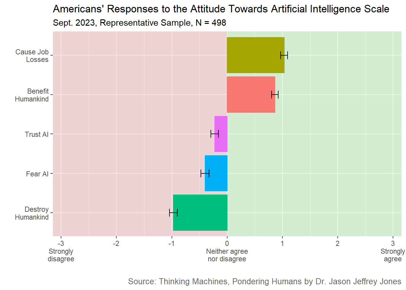
Figure 6.3: Attitude Towards Artificial Intelligence survey results. Plotted is mean response on a 7-point Likert scale from Strongly disagree to Strongly agree. Black bars are +/- one standard error.
The striking result is how close each mean is to the midpoint. Extreme attitudes toward AI were not common nor typical.
It is fun to note that here Americans agreed (weakly) that AI will “cause many job losses,” but when I asked directly about their own jobs, they were more sanguine - see Figure 4.1. Americans thought AI was coming for that guy’s job, not mine.
As we did before, let’s briefly ask how and if responses cluster. First, let’s examine the correlation matrix for the five items.
Code
# Select, label, and keep only the five ATAI items.ataiItems <- responses %>%select(starts_with("sinder_")) %>%rename(`Fear AI`= sinder_fear_ai,`Trust AI`= sinder_trust_ai,`Destroy Humankind`= sinder_destroy_humankind,`Benefit Humankind`= sinder_benefit_humankind,`Cause Job Losses`= sinder_job_losses ) %>%mutate(across(everything(), as.numeric))# Correlation matrix.ataiCor <-cor( ataiItems,use ="pairwise.complete.obs")# Reorder items so similar correlation profiles appear near each other.# This is not a substantive cluster model; it is just for figure readability.ataiOrder <-hclust(as.dist(1- ataiCor),method ="average")$labels[hclust(as.dist(1- ataiCor),method ="average" )$order]# Convert to long format for ggplot.ataiCorLong <- ataiCor %>%as.data.frame() %>%rownames_to_column("Item_1") %>%pivot_longer(cols =-Item_1,names_to ="Item_2",values_to ="Correlation" ) %>%mutate(Item_1 =factor(Item_1, levels = ataiOrder),Item_2 =factor(Item_2, levels =rev(ataiOrder)) )# Plot.ggplot(ataiCorLong, aes(x = Item_1, y = Item_2, fill = Correlation)) +geom_tile(color ="white", linewidth =0.5) +geom_text(aes(label =round(Correlation, 2)),size =3.5 ) +scale_fill_gradient2(low ="firebrick",mid ="white",high ="steelblue",midpoint =0,limits =c(-1, 1),breaks =seq(-1, 1, by =0.5) ) +scale_x_discrete(labels = \(x) stringr::str_wrap(x, width =12)) +scale_y_discrete(labels = \(x) stringr::str_wrap(x, width =12)) +coord_equal() +labs(title ="How Do Responses to the ATAI Items Cluster?",subtitle ="Items are ordered by similarity in their correlation profiles.",x ="",y ="",fill ="Correlation" ) +theme_minimal() +theme(axis.text.x =element_text(angle =45, hjust =1),panel.grid =element_blank(),legend.position ="right" )
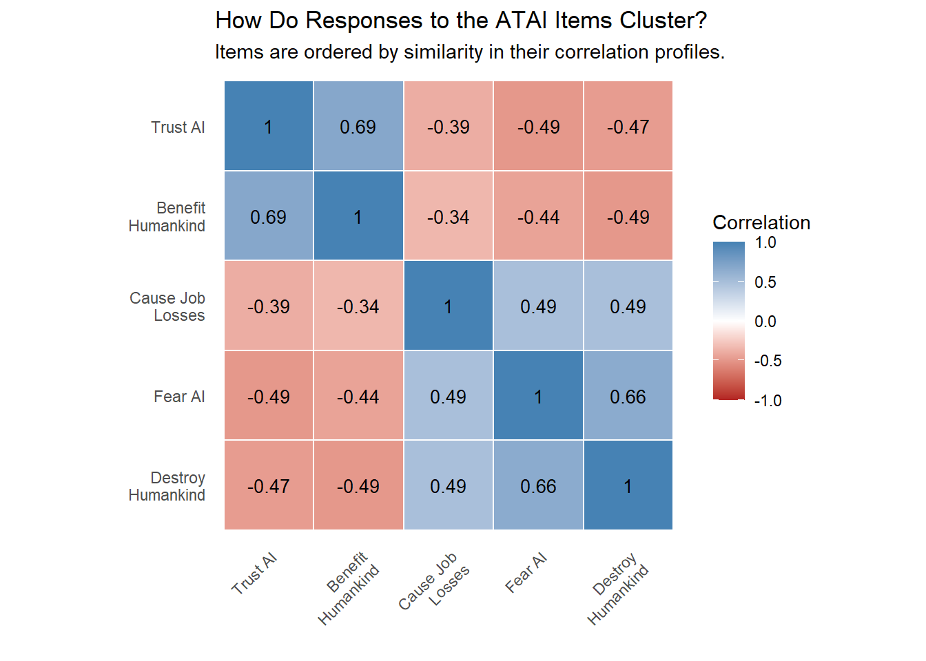
Figure 6.4: Correlation matrix for the five items in the Attitude Towards Artificial Intelligence scale. Knowing an individual’s response to any one item provided information on how they would respond to all others.
Hopefully, Figure 6.4 made you nod your head and slightly smile. It shows us the ATAI is a well-behaved scale. There are three items (Fear AI, Cause Job Losses and Destroy Humankind) that clearly measure negative attitude, and responses were similar across all three. Trust AI and Benefit Humankind reveal positive attitudes. Responses to these items correlate positively with each other and negatively with the negative items. The world makes sense.
Let us summarize and simplify, and at the same time further explore attitude scales. Twenty-five pair-wise correlations can be a bit much. What single number can answer the question: Has the scale adequately and reliably measured one construct? This number is Cronbach’s alpha. Cronbach’s alpha ranges from 0 to 1 — the closer to one, the more evidence there is that the scale consistently measures one latent variable. In our case, the latent variable is attitude toward AI.
After reverse-coding the negative items so that higher scores always indicate more positive attitudes toward AI, the five ATAI items showed good internal consistency, with Cronbach’s alpha = 0.83. This is great news. It means we can read Americans’ minds. Or a tiny sliver of their minds — specifically how positively (or negatively) they feel toward AI.
The high value of Cronbach’s alpha gives us license to treat the survey as a scale. We can place each respondent on an AI positivity number line by combining their five responses.
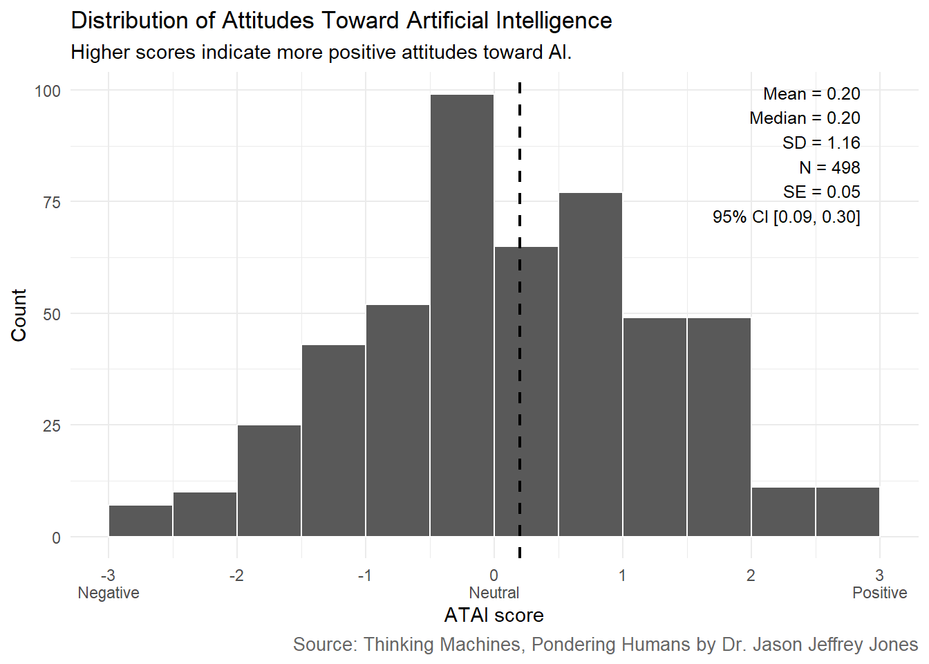
Figure 6.5: Distribution of respondent-level Attitude Towards Artificial Intelligence scores. Negative items were reverse-coded so that higher scores indicate more positive attitudes toward AI. Each respondent’s score is the mean of the five scored items, preserving the original -3 to +3 response scale.
Once again, we see that Americans felt mildly positive (but more middling than anything) toward AI in September 2023.
In our upcoming and final scale, I expect we will see more of the same. What do you predict?
6.1.2 AI Attitude Scale (AIAS-4 scale)
An optimistic, positive perspective is common to all four statements in the AIAS-4 scale. (See Section 6.2.1 for the exact wording.) Let’s examine to what degree Americans shared this perspective.
Code
# Select columns and pivot.aias4Responses <- responses %>%select(starts_with("grass_")) %>%pivot_longer(cols =everything(),names_to ="Item",names_prefix ="grass_",values_to ="Response" ) %>%mutate(Item =recode( Item,"improve_life"="AI will Improve My Life","improve_work"="AI will Improve My Work","use_in_future"="I Will Use AI","positive_humanity"="AI is Positive for Humanity" ) )# Summary figureaias4Responses %>%group_by(Item) %>%summarise(Mean_Response =mean(Response, na.rm =TRUE),sd =sd(Response, na.rm =TRUE),n =sum(!is.na(Response)),se = sd /sqrt(n),error_low = Mean_Response - se,error_high = Mean_Response + se ) %>%ggplot(aes(x =reorder(Item, Mean_Response), y = Mean_Response, color = Item, fill = Item)) +# Add green and red shading to demarcate agree vs disagree.annotate(geom="rect", xmin=-Inf, xmax=Inf, ymin=0.0, ymax=Inf, fill="green", alpha=0.1) +annotate(geom="rect", xmin=-Inf, xmax=Inf, ymin=-Inf, ymax=0.0, fill="red", alpha=0.1) +# Annotations go first, so data elements are layered on top.geom_col() +geom_errorbar(aes(ymin = error_low, ymax = error_high), color="black", width=0.2) +ggtitle("Americans' Responses to the AI Attitude Scale (AIAS-4) ", "Sept. 2023, Representative Sample, N = 498") +xlab("") +ylab("") +# Apply labels with wrapping.scale_x_discrete(labels =label_wrap(10)) +# Set color and fill values.# Force y scale to -3 through 3. Put numbers on y-axis. Add low and high labels.scale_y_continuous(limits =c(-3,3), breaks =-3:3, labels =c("-3\nStrongly\ndisagree", "-2", "-1", "0\nNeither agree\nnor disagree", "1", "2", "3\nStrongly\nagree"), expand=expansion(mult =0.025)) +labs(caption = book_source_caption) +theme(plot.caption =element_text(size=10, color ="#666666")) +# The legend has only redundant information. Get rid of it.theme(legend.position ="none") +coord_flip()
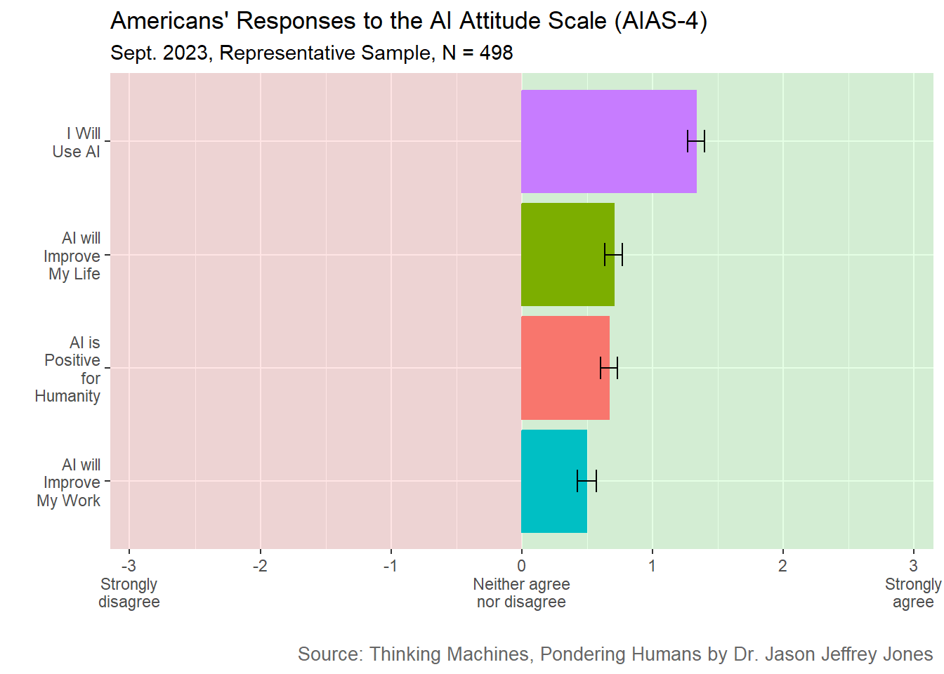
Figure 6.6: AI Attitude Scale survey results. Plotted is mean response on a 7-point Likert scale from Strongly disagree to Strongly agree. Black bars are +/- one standard error.
Cautious optimism once again. The strongest agreement was an intention to use AI in the future.
I have the intuition that responses to these items strongly correlate. It’s hard to imagine respondents who thought AI would improve their life but not be positive for humanity. Let’s examine a correlation matrix and alpha value.
Code
# Select, label, and keep only the five ATAI items.aias4Items <- responses %>%select(starts_with("grass_")) %>%rename(`Improve Life`= grass_improve_life,`Improve Work`= grass_improve_work,`Use in Future`= grass_use_in_future,`Positive Humanity`= grass_positive_humanity ) %>%mutate(across(everything(), as.numeric))# Correlation matrix.aias4Cor <-cor( aias4Items,use ="pairwise.complete.obs")# Reorder items so similar correlation profiles appear near each other.# This is not a substantive cluster model; it is just for figure readability.aias4Order <-hclust(as.dist(1- aias4Cor),method ="average")$labels[hclust(as.dist(1- aias4Cor),method ="average" )$order]# Convert to long format for ggplot.aias4CorLong <- aias4Cor %>%as.data.frame() %>%rownames_to_column("Item_1") %>%pivot_longer(cols =-Item_1,names_to ="Item_2",values_to ="Correlation" ) %>%mutate(Item_1 =factor(Item_1, levels = aias4Order),Item_2 =factor(Item_2, levels =rev(aias4Order)) )# Plot.ggplot(aias4CorLong, aes(x = Item_1, y = Item_2, fill = Correlation)) +geom_tile(color ="white", linewidth =0.5) +geom_text(aes(label =round(Correlation, 2)),size =3.5 ) +scale_fill_gradient2(low ="firebrick",mid ="white",high ="steelblue",midpoint =0,limits =c(-1, 1),breaks =seq(-1, 1, by =0.5) ) +scale_x_discrete(labels = \(x) stringr::str_wrap(x, width =12)) +scale_y_discrete(labels = \(x) stringr::str_wrap(x, width =12)) +coord_equal() +labs(title ="How Do Responses to the AIAS-4 Items Cluster?",subtitle ="Items are ordered by similarity in their correlation profiles.",x ="",y ="",fill ="Correlation" ) +theme_minimal() +theme(axis.text.x =element_text(angle =45, hjust =1),panel.grid =element_blank(),legend.position ="right" )
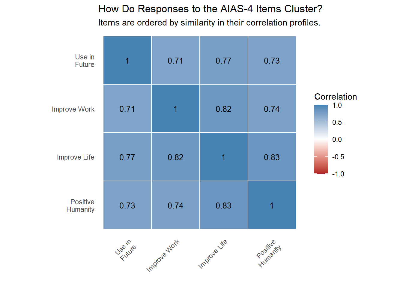
Figure 6.7: Correlation matrix for the four items in the AI Attitude Scale (AIAS-4). Knowing an individual’s response to any one item provided information on how they would respond to all others.
In the AIAS-4, every item correlates strongly and positive with every other item. Let’s view this first as success and then as failure.
If the goal of a scale is to use multiple probes (items) to measure one underlying construct, then the AIAS-4 is a success. The statements have face validity — they appear simple, easy to interpret and directly related to attitudes toward AI. They survey data confirms the intuition. Responses do not go off in all directions; agreeing with one item is a strong predictor you will agree with each of the others. The Cronbach’s alpha is extremely high: 0.93.
These same facts should lead to the conclusion the scale is a failure, however, once we acknowledge real-world constraints. Human survey response data is expensive to collect. The failure interpretation highlights the issue that we paid for four item responses, but all we really measured was one attitude!
Dealing with that constraint is the point of this chapter. Specifically, I want to ask and answer two questions:
Do we gain enough information running all three scales to justify the expense?
If we could only field one single item, which one should we choose?
6.1.3 Scale Showdown: How Many AI Attitude Items Do We Really Need?
There are two possibilities: The Lobera, ATAI and AIAS-4 scales each measure meaningfully different information, or I paid three times to hear the same answer. Let’s run some analysis to decide which better describes the data.
First, we will recode items so that positive numbers mean positive attitude and rescale items to z-scores.
Code
# Helper function: convert a variable to a z-score.z_score <-function(x) {as.numeric(scale(x))}ai_attitude_items <- responses %>%transmute(# Lobera items: original scale is 1 to 5.# Higher values should mean more positive attitude toward AI.lobera_benefits_scored =as.numeric(lobera_2020_ai_benes),lobera_risk_scored =6-as.numeric(lobera_2020_ai_risk),# ATAI items: original scale is -3 to +3.# Reverse-code negative items so higher values mean more positive attitude.atai_fear_ai_scored =-as.numeric(sinder_fear_ai),atai_trust_ai_scored =as.numeric(sinder_trust_ai),atai_destroy_humankind_scored =-as.numeric(sinder_destroy_humankind),atai_benefit_humankind_scored =as.numeric(sinder_benefit_humankind),atai_job_losses_scored =-as.numeric(sinder_job_losses),# AIAS-4 items: all are already positively keyed.aias4_improve_life_scored =as.numeric(grass_improve_life),aias4_improve_work_scored =as.numeric(grass_improve_work),aias4_use_in_future_scored =as.numeric(grass_use_in_future),aias4_positive_humanity_scored =as.numeric(grass_positive_humanity) )ai_attitude_items_z <- ai_attitude_items %>%mutate(across(everything(), z_score,.names ="{.col}_z" ) ) %>%select(ends_with("_z"))
Now, let’s find a score from each respondent on each scale. Then we’ll compare our 498 scale score triplets. If each score strongly predicts the two others, then I could have saved money by just running one scale and estimating the others.
Code
# Create respondent-level scale scores.# Because items are already z-scored, each scale score is the respondent's# average standardized response across that scale's items.ai_attitude_scale_scores <- ai_attitude_items_z %>%transmute(Lobera =rowMeans(select( ., lobera_benefits_scored_z, lobera_risk_scored_z ),na.rm =FALSE ),ATAI =rowMeans(select( ., atai_fear_ai_scored_z, atai_trust_ai_scored_z, atai_destroy_humankind_scored_z, atai_benefit_humankind_scored_z, atai_job_losses_scored_z ),na.rm =FALSE ),`AIAS-4`=rowMeans(select( ., aias4_improve_life_scored_z, aias4_improve_work_scored_z, aias4_use_in_future_scored_z, aias4_positive_humanity_scored_z ),na.rm =FALSE ) )# Convert to long format for programmatic modeling.scale_score_long <- ai_attitude_scale_scores %>%mutate(respondent_id =row_number()) %>%pivot_longer(cols =-respondent_id,names_to ="scale",values_to ="score" )# All ordered predictor/outcome scale pairs.scale_pairs <-expand_grid(outcome_scale =c("Lobera", "ATAI", "AIAS-4"),predictor_scale =c("Lobera", "ATAI", "AIAS-4")) %>%filter(outcome_scale != predictor_scale)# For each pair, regress outcome scale score on predictor scale score.pairwise_prediction_results <- scale_pairs %>%rowwise() %>%mutate(model_data =list( ai_attitude_scale_scores %>%select(outcome =all_of(outcome_scale),predictor =all_of(predictor_scale) ) %>%filter(!is.na(outcome), !is.na(predictor)) ),model =list(lm(outcome ~ predictor, data = model_data)),correlation =cor( model_data$outcome, model_data$predictor,use ="complete.obs" ),r_squared =summary(model)$r.squared,n =nrow(model_data) ) %>%ungroup() %>%select( predictor_scale, outcome_scale, n, correlation, r_squared ) %>%mutate(correlation =round(correlation, 2),r_squared =round(r_squared, 2) )pairwise_prediction_results %>%arrange(predictor_scale, outcome_scale) %>%kable(format ="markdown",col.names =c("Predictor Scale","Outcome Scale","N","Correlation","R-squared" ) )
Table 6.1
Predictor Scale
Outcome Scale
N
Correlation
R-squared
AIAS-4
ATAI
498
0.73
0.54
AIAS-4
Lobera
498
0.75
0.56
ATAI
AIAS-4
498
0.73
0.54
ATAI
Lobera
498
0.75
0.56
Lobera
AIAS-4
498
0.75
0.56
Lobera
ATAI
498
0.75
0.56
Examine the last two columns. Each scale correlates with both others. The R-squared values are strong, and no scale stands out as an outlier. This is fabulous news for the future and bad news for the past.
The fabulous news for the future is that one can choose any of the three scales. With survey data from only the ATAI scale, you can calculate a very good guess about what your respondents would have scored had you given them the AIAS-4. And it’s the same in the other direction, too.
The bad news for the past isn’t even that bad. As far as I am concerned, the table above tells me that any of the three scales serves as a drop-in replacement for any of the others. So, yes I did overpay. But we only know that because I ran all three scales on the same sample.
Let’s move on to true efficiency. If one could only field a single item (not the whole scale), which single item is the best choice?
For each item, let’s calculate how well that one item predicts the average of the other ten items.
Code
# Human-readable labels for the 11 candidate items.item_labels <-tibble(item =c("lobera_benefits_scored_z","lobera_risk_scored_z","atai_fear_ai_scored_z","atai_trust_ai_scored_z","atai_destroy_humankind_scored_z","atai_benefit_humankind_scored_z","atai_job_losses_scored_z","aias4_improve_life_scored_z","aias4_improve_work_scored_z","aias4_use_in_future_scored_z","aias4_positive_humanity_scored_z" ),scale =c("Lobera","Lobera","ATAI","ATAI","ATAI","ATAI","ATAI","AIAS-4","AIAS-4","AIAS-4","AIAS-4" ),item_label =c("Benefits","Risk (reverse-coded)","Fear (reverse-coded)","Trust","Destroy humankind (reverse-coded)","Benefit humankind","Job losses (reverse-coded)","Improve my life","Improve my work","Use in future","Positive for humanity" ))single_item_prediction <-function(candidate_item) { other_items <-setdiff(names(ai_attitude_items_z), candidate_item ) model_data <- ai_attitude_items_z %>%mutate(single_item = .data[[candidate_item]],other_items_composite =rowMeans(select(., all_of(other_items)),na.rm =FALSE ) ) %>%select(single_item, other_items_composite) %>%filter(!is.na(single_item), !is.na(other_items_composite)) model <-lm(other_items_composite ~ single_item, data = model_data)tibble(item = candidate_item,n =nrow(model_data),correlation_with_other_items =cor( model_data$single_item, model_data$other_items_composite,use ="complete.obs" ),r_squared =summary(model)$r.squared )}single_item_efficiency <-map_dfr( item_labels$item, single_item_prediction) %>%left_join(item_labels, by ="item") %>%mutate(correlation_with_other_items =round(correlation_with_other_items, 2),r_squared =round(r_squared, 2) ) %>%arrange(desc(r_squared)) %>%select( scale, item_label, n, correlation_with_other_items, r_squared )single_item_efficiency %>%mutate(item_label =fct_reorder(item_label, r_squared) ) %>%ggplot(aes(x = item_label, y = r_squared, fill = scale)) +geom_col() +geom_text(aes(label =sprintf("%.2f", r_squared)),hjust =-0.1,size =3.25 ) +coord_flip() +scale_y_continuous(limits =c(0, max(single_item_efficiency$r_squared) +0.08),breaks =seq(0, 1, by =0.1) ) +labs(title ="Which Single Item Best Recovers the Full AI Attitude Battery?",subtitle ="Each item predicts the average of the other ten items.",x ="",y ="R-squared",fill ="Original scale",caption = book_source_caption ) +theme_minimal() +theme(panel.grid.minor =element_blank(),plot.caption =element_text(size =10, color ="#666666") )
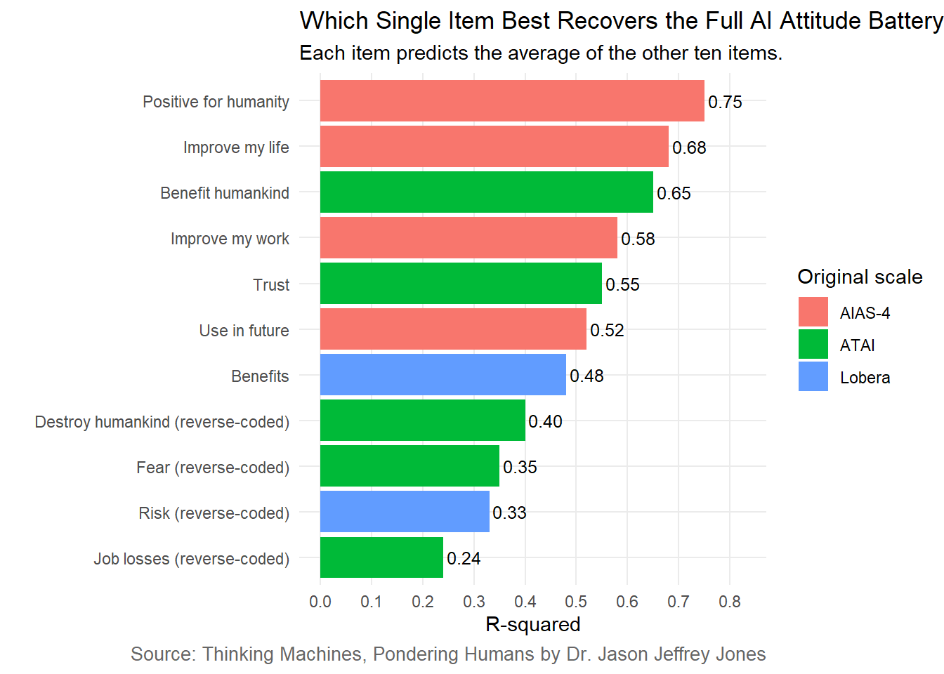
Figure 6.8: Efficiency of each AI attitude item as a one-item measure. Each bar shows how well one item predicts the average of the other ten positively keyed, z-scored items.
Our winning item:
I think artificial intelligence technology is positive for humanity.
Who best predicted the average response to the other ten items? I think artificial intelligence technology is positive for humanity. Perhaps we should have predicted this. This item is explicitly valenced and general. It avoids being too entangled with personal employment and personal use. It is not speculation about a specific extreme apocalyptic outcome.
Of course, humans’ views on all of these things are interesting and valuable. But survey funding is limited. This dilemma led me to my current ambition: Leading a Golden Age of Surveys.
6.2 Survey Items, Respondents and Costs
6.2.1 Survey Items
The survey contained all items from three different AI attitude scales. Every respondent responded to every item. The survey software chose a random order of items for each respondent.
Below is the exact wording of each item.
Using a scale of 1 to 5, where 1 means no risk and 5 means many risks, to what extent do you think there are risks in artificial intelligence?
lobera_2020_ai_benes Using a scale of 1 to 5, where 1 means no benefit and 5 means many benefits, to what extent do you think artificial intelligence has benefits?
The two Lobera et al. items specified a 1 to 5 response scale. The remaining items did not. Respondents chose one of seven points, ranging from Strongly disagree to Strongly agree.
I fear artificial intelligence.
I trust artificial intelligence.
Artificial intelligence will destroy humankind.
Artificial intelligence will benefit humankind.
Artificial intelligence will cause many job losses.
Respondents were recruited through Prolific Academic. I requested a representative sample of 500 American adults. Specifically, I chose the option “USA, Factors: Sex, Age, Ethnicity (Simplified US Census).” Two respondents had no matching demographic profile and were dropped.
The study was run once September 14-17, 2023.
To demonstrate the demographic coverage, below I provide the Sex and Age crosstab:
Code
# Bin ages.demosTable2023Scales = responses %>%rename(Age_Raw = Age) %>%select(Sex, Age_Raw)demosTable2023Scales = demosTable2023Scales %>%mutate(Age ="UNKNOWN" ) %>%mutate(Age =if_else(Age_Raw >=18& Age_Raw <25, "18-24", Age) ) %>%mutate(Age =if_else(Age_Raw >=25& Age_Raw <35, "25-34", Age) ) %>%mutate(Age =if_else(Age_Raw >=35& Age_Raw <45, "35-44", Age) ) %>%mutate(Age =if_else(Age_Raw >=45& Age_Raw <55, "45-54", Age) ) %>%mutate(Age =if_else(Age_Raw >=55& Age_Raw <65, "55-64", Age) ) %>%mutate(Age =if_else(Age_Raw >=65, "65+", Age) )# Generate percentage per demographic bin for each survey sample.demosTable2023Scales = demosTable2023Scales %>%filter(!is.na(Sex), !is.na(Age)) %>%group_by(Sex, Age) %>%summarise(groupN =n() ) %>%# Add totalN.ungroup() %>%mutate(totalN =sum(groupN) ) %>%# Now we can divide across each row to calculate a percentage.mutate(percent =round(100* groupN / totalN, 0) ) %>%select(-totalN)kable(demosTable2023Scales, format ="markdown")
Table 6.2
Sex
Age
groupN
percent
Female
18-24
36
7
Female
25-34
40
8
Female
35-44
45
9
Female
45-54
44
9
Female
55-64
56
11
Female
65+
37
7
Male
18-24
29
6
Male
25-34
49
10
Male
35-44
42
8
Male
45-54
43
9
Male
55-64
52
10
Male
65+
25
5
6.2.3 Costs
The survey took 3 minutes. Each respondent was paid $0.60. Thus, the total of payments to respondents was $300 = 500 * $0.60.
Prolific Academic charged a Service fee equal to 33% of respondent payments. This totaled $99.99.
During this time, Prolific waived the Representative sample fee.
R code for analysis and visualization is embedded above (some formats) or available at TODO GITHUB/ZENODO.
6.4 Summary and What’s Next
The main findings of this chapter deserve repetition:
Extreme attitudes toward AI were not common nor typical.
You can measure attitude toward AI in different ways and arrive at the same result.
A single item can recover much of the signal in an entire scale.
Representative sample surveys prove their worth again in this chapter. If one’s sources were social media, editorials and online videos, I believe it would be easy to have mistakenly believed the opposite of #1 above. That content was created with the goal of eliciting strong reactions, and the more engagement the content received, the wider an audience it reached. Hype and its backlash were visible, while common opinion was invisible (except to surveys).
The mushy middle reality of Figure 6.2 and Figure 6.3 was not engaging content. “Americans had weakly positive feelings” did not go viral. It just happens to be the truth.
Let’s recall that I fielded these surveys in September 2023. Many individuals had little experience with generative AI. Google Bard and Microsoft Bing Chat — both already forgotten by 2026 — were still flagship products. It’s easy to imagine attitudes toward AI were inchoate at that time.
Wouldn’t it be fantastic, then, if someone began consistently and persistently measuring those attitudes? If you are screaming YES, get on with it! at your screen, then your next stop should be Leading a Golden Age of Surveys. In that chapter, I further pursue the idea of single-item surveying. I needed the efficiency of that approach to initiate daily surveys. We will see that time does make a difference.
Otherwise, let’s continue examining American public opinion early in the Gen AI Age: with repeated survey experiments, we’ll examine what worried Americans about AI and other technologies.