9How did attitudes toward AI compare to other technologies?
Artificial intelligence doesn’t exist in a vacuum. There are many developing technologies, and money is a limited resource. In this chapter, we will compare opposition and support for AI to other technologies.
I used the method of a survey experiment again. Respondents were asked how much they opposed or supported government funding for further development. AI was one of eleven technologies.
9.1 Analysis, Visualization and Interpretation
Section 8.1.2 introduced and quantified AI Support. Here, let’s place AI Support in context.
In this survey, I wanted respondents to prioritize (at least implicitly). That is why I asked about government funding, probed for opposition versus support, and included technologies I hypothesized would range in popularity.
Code
# The file ai-versus-2023-wide-correlates.csv contains responses# from a US representative sample of 500 respondents.# Download the file from a public repository at# https://doi.org/10.5281/zenodo.20399282responses =read_csv("data/ai-versus-2023-wide-correlates.csv")# Reader-friendly labels for the support targets.support_labels <-c(oppose_or_support_space_exploration ="Space exploration",oppose_or_support_quantum_computing ="Quantum computing",oppose_or_support_carbon_removal ="Carbon removal",oppose_or_support_virtual_reality ="Virtual reality",oppose_or_support_self_driving_cars ="Self-driving cars",oppose_or_support_ai ="Artificial intelligence",oppose_or_support_geoengineering ="Geoengineering",oppose_or_support_facial_recognition ="Facial recognition",oppose_or_support_genetic_editing_humans ="Genetic editing of humans",oppose_or_support_personalized_advertising ="Personalized advertising",oppose_or_support_cryptocurrency ="Cryptocurrency")# Highlight AI; keep the comparison technologies visually secondary.support_colors <-setNames(rep("gray50", length(support_labels)),unname(support_labels))support_colors["Artificial intelligence"] <-"#4DAF4A"# Convert from one row per respondent to one row per# respondent-technology combination, then calculate mean support# and its 95% confidence interval.support_summary <- responses %>%select(all_of(names(support_labels))) %>%pivot_longer(cols =everything(),names_to ="technology",values_to ="support" ) %>%mutate(technology =factor( technology,levels =names(support_labels),labels =unname(support_labels) ) ) %>%group_by(technology) %>%summarise(n =sum(!is.na(support)),mean_support =mean(support, na.rm =TRUE),se =sd(support, na.rm =TRUE) /sqrt(n),ci_low = mean_support -qt(.975, df = n -1) * se,ci_high = mean_support +qt(.975, df = n -1) * se,.groups ="drop" ) %>%mutate(technology =fct_reorder(technology, mean_support) )book_source_caption =paste0("Source: Thinking Machines, Pondering Humans by Dr. Jason Jeffrey Jones")support_caption <-paste0("Points show mean support. Bars show 95% confidence intervals.\n","Responses range from −3 (Strongly oppose) to +3 (Strongly support).\n", book_source_caption)# Plot mean support and 95% confidence intervals.ggplot( support_summary,aes(x = mean_support,y = technology,color = technology )) +geom_vline(xintercept =0,linetype ="dashed",color ="gray70" ) +geom_segment(aes(x = ci_low,xend = ci_high,yend = technology ),linewidth =0.8 ) +geom_point(size =3) +scale_color_manual(values = support_colors,guide ="none" ) +scale_x_continuous(breaks =-3:3,limits =c(-3, 3) ) +labs(title ="How much do you oppose or support government funding\nfor the further development of...?",subtitle ="US Adults, Representative sample, N=500. Surveyed Sept. 2023",x ="Mean opposition (−3) or support (+3)",y =NULL,caption = support_caption ) +theme_minimal() +theme(panel.grid.minor =element_blank(),panel.grid.major.y =element_blank(),plot.caption =element_text(size =10,color ="#666666",hjust =1 ) )
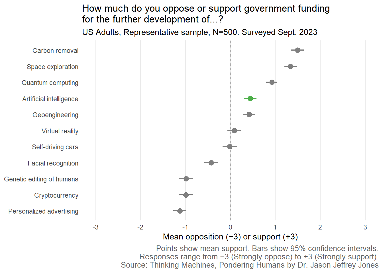
Figure 9.1: Mean opposition or support for funding across targets in the 2023 survey experiment. For each technology respondents answered ‘How much do you oppose or support government funding for the further development?’ on a seven-point scale. Error bars show 95% confidence intervals.
Figure 9.1 demonstrates that a few technologies were more strongly supported than AI. Carbon removal, Space exploration, and Quantum computing received the highest mean support. AI and Geoengineering ranked next, and average support was greater than zero.
US government funding was crucial in early development of self-driving cars. In 2023, Americans were lukewarm about that application, however. Perhaps because they saw for-profit companies already developing and deploying their own autonomous vehicles. Similarly, respondents may have been unenthusiastic about virtual reality, because they saw it as a consumer product already.
But wait. Does that argument work? In September 2023, ChatGPT was a consumer AI product with tens of millions of users. TODO finish thoughts
9.2 Survey Items, Respondents and Costs
9.2.1 Survey Items
The intent of this survey was to contrast Americans’ support for government funding across several technologies.
On a seven-point scale, respondents were asked how much they opposed or supported “government funding for the further development.” The order of the technologies was randomly chosen for each respondent.
How much do you oppose or support government funding for the further development of each technology?
artificial intelligence
carbon removal
cryptocurrency
facial recognition
genetic editing of humans
geoengineering
personalized advertising
quantum computing
self-driving cars
space exploration
virtual reality
In order to place AI Support in context, I chose techs I hypothesized would be popular (e.g. space exploration) and those I hypothesized would be unpopular (e.g. personalized advertising).
Each respondent reported a level of funding opposition or support for every technology.
Other items measured generalized trust and risk preference:
Generally speaking, would you say that most people can be trusted or that you can’t be too careful in dealing with people?
How do you see yourself: are you generally a person who is fully prepared to take risks or do you try to avoid taking risks? Please choose a number, where the value 0 means: ‘not at all willing to take risks’ and the value 10 means: ‘very willing to take risks’.
9.2.2 Respondents
Respondents were recruited through Prolific Academic. I requested a representative sample of 500 American adults. Specifically, I chose the option “USA, Factors: Sex, Age, Ethnicity (Simplified US Census).”
To demonstrate the demographic coverage, below I provide the Sex and Age crosstab for this 2023 sample:
Code
library(knitr)# Bin ages.demosTable2023Versus = responses %>%rename(Age_Raw = Age) %>%select(Sex, Age_Raw)demosTable2023Versus = demosTable2023Versus %>%mutate(Age ="UNKNOWN" ) %>%mutate(Age =if_else(Age_Raw >=18& Age_Raw <25, "18-24", Age) ) %>%mutate(Age =if_else(Age_Raw >=25& Age_Raw <35, "25-34", Age) ) %>%mutate(Age =if_else(Age_Raw >=35& Age_Raw <45, "35-44", Age) ) %>%mutate(Age =if_else(Age_Raw >=45& Age_Raw <55, "45-54", Age) ) %>%mutate(Age =if_else(Age_Raw >=55& Age_Raw <65, "55-64", Age) ) %>%mutate(Age =if_else(Age_Raw >=65, "65+", Age) )# Generate percentage per demographic bin for each survey sample.demosTable2023Versus = demosTable2023Versus %>%filter(!is.na(Sex), !is.na(Age)) %>%group_by(Sex, Age) %>%summarise(N =n() ) %>%# Add totalN.ungroup() %>%mutate(totalN =sum(N) ) %>%# Now we can divide across each row to calculate a percentage.mutate(percent =round(100* N / totalN, 0) ) %>%select(-totalN)kable(demosTable2023Versus, format ="markdown")
Table 9.1
Sex
Age
N
percent
Female
18-24
20
4
Female
25-34
60
12
Female
35-44
40
8
Female
45-54
38
8
Female
55-64
67
13
Female
65+
33
7
Male
18-24
14
3
Male
25-34
54
11
Male
35-44
59
12
Male
45-54
31
6
Male
55-64
43
9
Male
65+
41
8
9.2.3 Costs
Each respondent was paid $0.60. Thus, the total of payments to respondents was $300 = 500 * $0.60.
Prolific Academic charged a Service fee equal to 33% of respondent payments. This totaled $100.
During this time, Prolific waived the Representative sample fee.