So far, we have only analyzed data from users in the United States. The Twitter data was sampled from everywhere, however. Why not extend our analyses to more nations?
We can begin with similar places. Australia, Canada and the United Kingdom share the primary language of English with the US. I would expect to see most trends observed in the US also present in these countries because of the strong web of influence the cultures are enmeshed in. Let’s recreate Figure 3.2 for each of these nations.
Code
library(tidyverse)# Download a csv file containing multinational data for tokens at annual resolution.# Read about the data in the text file at https://osf.io/mdp7k# HINENI stands for Human Identity across Nations of the Earth Ngram Investigator.hineni =read_csv("https://osf.io/download/k7bwj/")# Become familiar with the data file.str(hineni) # Structure of the data.hineni %>%slice_sample(n =5) # Example rows.# How many users include the word vegan in their Twitter profile?hineni %>%filter(ngram =="vegan"& obsYear ==2012) # in 2012hineni %>%filter(ngram =="vegan"& obsYear ==2020) # in 2020# Note that the numerator column contains the incidence.
Code
hineni %>%filter(ngram %in%c("vegan", "vegetarian", "carnivore") ) %>%filter(nation %in%c("AU", "CA", "GB", "US") ) %>%mutate(Nation =factor(nation, levels =c("AU", "CA", "GB", "US"), labels =c("Australia", "Canada", "United Kingdom", "United States")) ) %>%mutate(finePrevalence =10000* numerator / denominator ) %>%mutate(Signifier =factor(ngram, levels =c("vegan", "vegetarian", "carnivore")) ) %>%ggplot(aes(x = obsYear, y = finePrevalence, color = Signifier, shape = Signifier)) +geom_path(linetype ="longdash", linewidth =1) +geom_point(size=4) +scale_x_continuous(breaks =seq(2012, 2023, 2)) +scale_color_manual(values =c("#5c8326", "#B61500", "#a16868") ) +ggtitle("Estimated prevalence of food-related signifiers", "within AU, CA, UK and US Twitter users' bios 2012-2023") +xlab("Year") +ylab("Prevalence\n(per 10,000 accounts)") +facet_wrap(vars(Nation), nrow =2) +theme(axis.text.x =element_text(angle =45, hjust =1) ) +theme(text =element_text(size=16)) +theme(legend.background =element_rect(fill ="white", color ="black")) +labs(caption ="Source: Ipseology - a new science of the self\n \uA9 Jason Jeffrey Jones.\nYou may share and adapt this work under terms of the CC BY 4.0 License.") +theme(plot.caption =element_text(size=10, color ="#666666"))
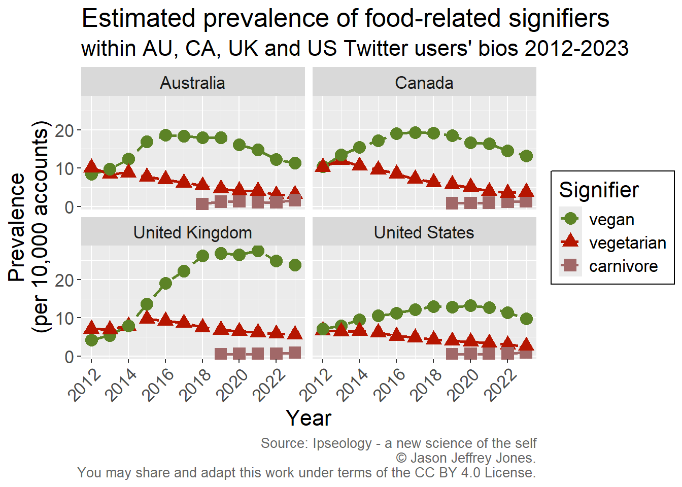
Figure 4.1: Prevalence of vegan, vegetarian and carnivore over time in Australia, Canada, the United Kingdom and the United States.
We see the same pattern in each country: vegan growth and vegetarian decline. Compared to the United States, the rise of vegan was more vigorous in Australia, Canada and especially the United Kingdom.
4.2 Use previous analysis as a template.
We begin to see the utility of the ipseological approach. When we measure consistently, persistently and precisely at scale, comparisons across time and space become accessible.
Let’s use our previous analysis as a template for more. There are several primarily Spanish-speaking nations in the data. Why not try a simple extension? Google Translate tells me there are feminine and masculine forms of vegan (vegana, vegano) and similarly for vegetarian (vegetariana, vegetariano). How popular was each of these across years and nations?
Code
hineni %>%filter(ngram %in%c("vegano", "vegana", "vegetariano", "vegetariana") ) %>%filter(nation %in%c("AR", "CL", "CO", "MX", "PE", "ES", "VE") ) %>%mutate(Gender =if_else(ngram %in%c("vegana", "vegetariana"), "Fem", "Masc") ) %>%mutate(Nation =factor(nation, levels =c("AR", "CL", "CO", "MX", "PE", "ES", "VE"), labels =c("Argentina", "Chile", "Colombia", "Mexico", "Peru", "Spain", "Venezuala")) ) %>%mutate(finePrevalence =10000* numerator / denominator ) %>%mutate(Signifier =factor(ngram, levels =c("vegano", "vegana", "vegetariano", "vegetariana")) ) %>%# Get rid of Chile.#filter(Nation != "Chile" ) %>% ggplot(aes(x = obsYear, y = finePrevalence, color = Signifier, shape = Signifier)) +geom_path(linetype ="dashed", linewidth =0.75) +geom_point(size=2) +scale_x_continuous(breaks =seq(2012, 2023, 2)) +#scale_y_continuous(limits = c(0,6), breaks = seq(0, 6, 2), expand = expansion(add=c(0.5, 2)) ) +scale_color_manual(values =c("#5c8326", "#5c8326", "#B61500", "#B61500") ) +ggtitle("Estimated prevalence of food-related signifiers", "within some Spanish-speaking nations' Twitter users' profile bios 2012-2023") +xlab("Year") +ylab("Prevalence\n(per 10,000 accounts)") +facet_grid(rows =vars(Nation), cols =vars(Gender) ) +# , scales = "free_y"theme(axis.text.x =element_text(angle =45, hjust =1) ) +#theme(text = element_text(size=16)) +theme(strip.text.y =element_text(angle =0) ) +#theme(panel.spacing.y = unit(2, "lines") ) +theme(legend.background =element_rect(fill ="white", color ="black")) +labs(caption ="Source: Ipseology - a new science of the self\n \uA9 Jason Jeffrey Jones.\nYou may share and adapt this work under terms of the CC BY 4.0 License.") +theme(plot.caption =element_text(size=10, color ="#666666"))
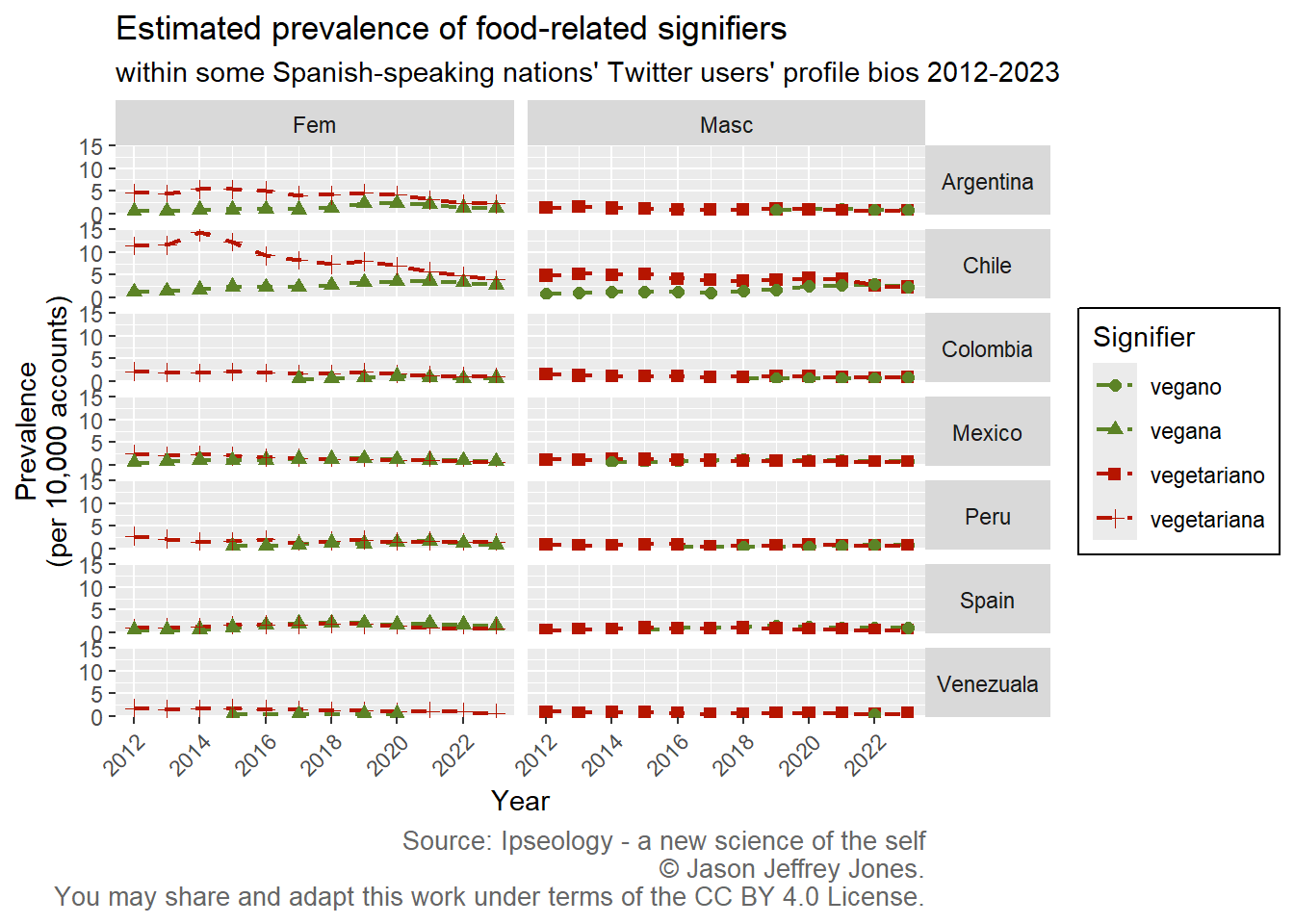
Figure 4.2: Prevalence of feminine and masculine forms of vegan and vegetarian over time in some Spanish-speaking nations.
This is not the most beautiful figure, but it tells us quite a bit. Our chosen signifiers - vegano, vegana, vegetariano, vegetariana saw infrequent use. Prevalence was in the low single digits with the exceptions of early years vegetariana in Chile.
Some (not many) define themselves by what they eat. How about what one plays or watches?
4.3 The multinational ipseology of soccer.
Let’s stick with Spanish-speaking nations and examine two ways individuals might signify their interest in what Pelé called the beautiful game: fútbol and the :soccer: emoji.
Code
# Load emojis from file.library(emoji)soccerTokens =c("fútbol", emoji('soccer'))hineni %>%filter(ngram %in% soccerTokens ) %>%filter(nation %in%c("AR", "CL", "CO", "MX", "PE", "ES", "VE") ) %>%mutate(Nation =factor(nation, levels =c("AR", "CL", "CO", "MX", "PE", "ES", "VE"), labels =c("Argentina", "Chile", "Colombia", "Mexico", "Peru", "Spain", "Venezuala")) ) %>%mutate(finePrevalence =10000* numerator / denominator ) %>%mutate(Signifier =factor(ngram, levels = soccerTokens) ) %>%ggplot(aes(x = obsYear, y = finePrevalence, color = Signifier, shape = Signifier)) +geom_path(linetype ="dashed", linewidth =0.75) +geom_point(size=2) +scale_x_continuous(breaks =seq(2012, 2023, 2)) +#scale_y_continuous(limits = c(0,6), breaks = seq(0, 6, 2), expand = expansion(add=c(0.5, 2)) ) +#scale_color_manual(values = c("#5c8326", "#5c8326", "#B61500", "#B61500") ) +ggtitle("Estimated prevalence of fútbol signifiers", "within some Spanish-speaking nations' Twitter users' profile bios 2012-2023") +xlab("Year") +ylab("Prevalence\n(per 10,000 accounts)") +facet_wrap(vars(Nation), nrow =3) +# , scales = "free_y"theme(axis.text.x =element_text(angle =45, hjust =1) ) +#theme(text = element_text(size=16)) +theme(strip.text.y =element_text(angle =0) ) +#theme(panel.spacing.y = unit(2, "lines") ) +theme(legend.background =element_rect(fill ="white", color ="black")) +labs(caption ="Source: Ipseology - a new science of the self\n \uA9 Jason Jeffrey Jones.\nYou may share and adapt this work under terms of the CC BY 4.0 License.") +theme(plot.caption =element_text(size=10, color ="#666666"))
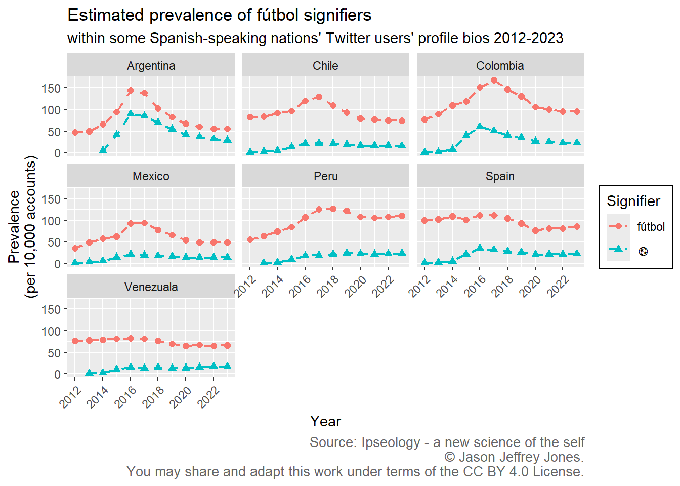
Figure 4.3: Prevalence of soccer-related signifiers in some Spanish-speaking nations.
Note that the maximum on the y-axis for fútbol is 10x what it was for vegetariana. As ipseologists, we can interpret this difference. Individuals in these countries are vastly more likely to mention a soccer interest as compared to a vegetarian status.
Individuals with fútbol in the bio outnumber those with the :soccer: emoji in every country and every year. But emojis offer something very compelling. They are language-independent. An arduous way to continue our multinational examination of soccer would be to translate into each language: Fußball, voetbal, 축구, etc. Let’s take a different tack, and follow the wind of emoji instead.
4.4 Emojis are language-independent but not context-independent.
Sometimes language differences are exactly what we are interested in; sometimes they just get in the way. Thankfully, there are emojis.
Emojis are language-independent but not context-independent. They are meant to represent the same thing no matter the language or nation they are embedded in. But certainly, some emojis are more personally meaningful to individuals in some contexts compared to others.
In the previous section, we saw some evidence that many individuals in Spanish-speaking nations mention fútbol in their self-descriptions. How common is a soccer affinity generally over other nations? How about other sports? Let’s use emoji representations of sports to find out.
We have the luxury of data for 32 nations, but let’s not generate 32 different graphs times 12 years. Instead, let’s choose one year (2022) and a reasonable set of sports emojis: ⚽, 🏀, ⚾, 🏏, 🏈, ⛳, 🎾.
Now let’s visualize the relative popularity of each sport emoji within bios in all these nations.
Code
sportsEmojis =c(emoji('soccer'), emoji('basketball'), emoji('baseball'), emoji('cricket game'), emoji('football'), emoji('golf'), emoji('tennis') )#sportsEmojisColors = c(emoji('soccer') = "#333333", emoji('basketball') = "#ee6730", emoji('baseball') = "#000089", emoji('cricket') = "#d6b268", emoji('football') = "#663831", emoji('golf') = "#0c8c3e", emoji('tennis') = "#cd3464" )sportsEmojisColors2 =c("#333333", "#ee6730", "#000089", "#d6b268", "#663831", "#0c8c3e", "#cd3464" )sportsEmojisColors2 =setNames(sportsEmojisColors2, sportsEmojis)# Download a file mapping nation abbreviations to nation names.nationList =read_csv("https://osf.io/download/qat5c/")nationList = nationList %>%mutate(nationName =factor(nationName) )hineni %>%filter(obsYear ==2022) %>%filter(ngram %in% sportsEmojis ) %>%mutate(Signifier =factor(ngram, levels = sportsEmojis) ) %>%# Join in nationList.mutate(nationCode = nation ) %>%inner_join(nationList) %>%group_by(nationName) %>%mutate(proportion = numerator /sum(numerator)) %>%ungroup() %>%# Order the nationName factor alphabetically.mutate(nationName =factor(nationName, levels =sort(unique(nationName), decreasing =TRUE)) ) %>%ggplot(aes(x = proportion, y = nationName, fill = Signifier)) +geom_bar(stat ="identity") +scale_fill_manual(values = sportsEmojisColors2 ) +scale_x_continuous(expand =c(0, 0)) +ggtitle("Proportion of sports emojis per sport per nation", "within each nation's Twitter users' profile bios in 2022") +xlab("Proportion") +ylab(NULL) +labs(caption ="Source: Ipseology - a new science of the self\n \uA9 Jason Jeffrey Jones.\nYou may share and adapt this work under terms of the CC BY 4.0 License.") +theme(plot.caption =element_text(size=10, color ="#666666"))
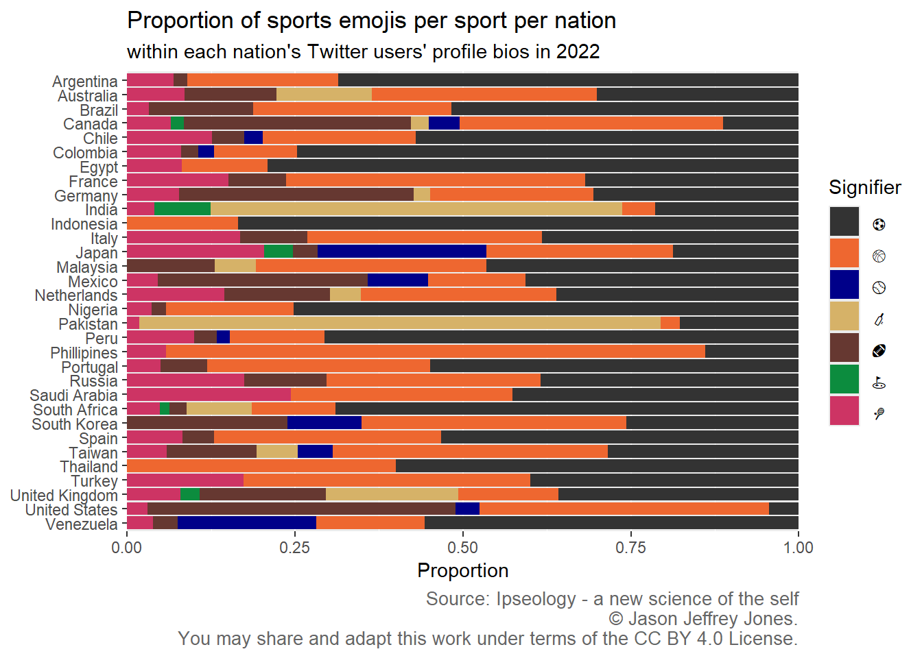
Figure 4.4: Relative popularity of each sport among users in each nation that include a sports emoji in their bio. Find a nation name on the left, and scan across to see the proportions for each sport. Cricket is popular in India, Pakistan and a few other nations. Soccer is widely popular, except in the US, where it is crowded out by basketball and American football.
The people of earth sure love soccer. In more than half of these nations, ⚽ is the most popular sports emoji users place within their bios.
There are so many more emojis to explore. It just so happened I was thinking about soccer and football when I wrote this chapter. Already, I hope you have thought of more interesting comparisons to make across time and geography. I have tried to make that an easy project to get started on, as you’ll see in the next section introducing HINENI.
4.5 Explore with HINENI.
HINENI stands for Human Identities across Nations of the Earth Ngram Investigator. HINENI comprises a dataset and tools allowing anyone to explore the popularity of signifiers within profile bios. It covers 32 nations and the years 2012 through 2023.