In ipseology, a bio revision event occurs when one observes a change over time in the set of signifiers an individual chooses to include in their self-description. In this Chapter, we’ll come to understand the four possible bio revision events: Add, Delete, Keep and Ignore.
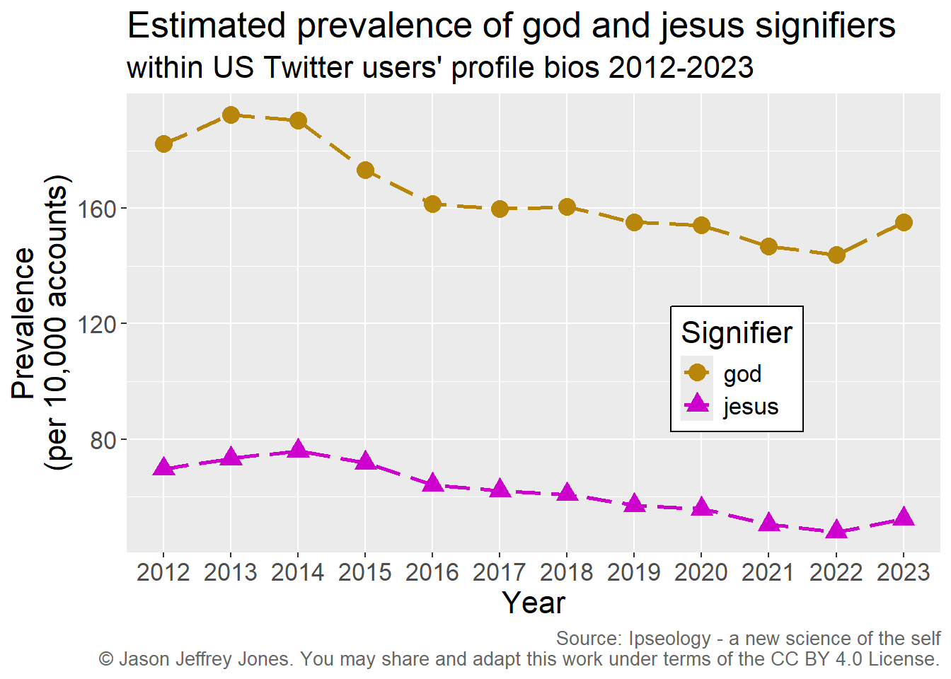
Let’s use religious signifiers in the United States as our domain of study. There are many signifiers we might use; let’s begin with only two for simplicity: god and jesus. As Figure 5.1 illustrates, these were consistently popular signifiers within US users’ bios. (In 2022, god was the 86th most popular token and more popular than 99.4% of all other tokens; jesus was more popular than 97.9% of all other tokens.)
Code
library(tidyverse)# Download a csv file containing US data for tokens at annual resolution.# Read about the data in the text file at https://osf.io/3gjtatac =read_csv("https://osf.io/download/cdzsb/")# Compute finePrevalence and begin years at 2012.tac= tac %>%filter(obsYear >2011) %>%mutate(finePrevalence =10000* numerator / denominator )# For the text, find rankings.godJesus2022Ranks = tac %>%filter(obsYear ==2022) %>%mutate(rowNum =row_number(-finePrevalence) ) %>%mutate(minRank =min_rank(-finePrevalence) ) %>%mutate(denseRank =dense_rank(-finePrevalence) ) %>%mutate(percentRank =percent_rank(finePrevalence) ) %>%mutate(cumeDist =cume_dist(finePrevalence) ) %>%filter(token %in%c("god", "jesus") )# Visualize god and jesus prevalence over time.tac %>%filter(token %in%c("god", "jesus") ) %>%mutate(Signifier =factor(token, levels =c("god", "jesus")) ) %>%ggplot(aes(x = obsYear, y = finePrevalence, color = Signifier, shape = Signifier)) +geom_path(linetype ="longdash", linewidth =1) +geom_point(size=4) +scale_x_continuous(limits=c(2012,2023), breaks =2012:2023, minor_breaks =NULL) +scale_color_manual(values =c("darkgoldenrod", "magenta3")) +ggtitle("Estimated prevalence of god and jesus signifiers", "within US Twitter users' profile bios 2012-2023") +xlab("Year") +ylab("Prevalence\n(per 10,000 accounts)") +theme(text =element_text(size=16)) +theme(legend.position =c(0.75, 0.4),legend.background =element_rect(fill ="white", color ="black")) +labs(caption ="Source: Ipseology - a new science of the self\n \uA9 Jason Jeffrey Jones. You may share and adapt this work under terms of the CC BY 4.0 License.") +theme(plot.caption =element_text(size=10, color ="#666666"))
Figure 5.1: Prevalence of god and jesus signifiers in US bios over time.
We see that prevalence of god and jesus ended at lower values than they began. One would rightfully wonder if users are deleting these words from their bios. However, from cross-sectional analysis it is impossible to know. We must use longitudinal analysis - in which we observe the same users’ bios at different times - to observe and tally bio revision events.
Keeping it simple again, let’s consider every possibility for god when we observe one user’s bio exactly twice.
Illustrating bio revision events for god
Early Bio
Late Bio
God Events
All glory to Jesus!
All glory to God!
Add God
All glory to God!
All glory to Tom Brady!
Delete God
All glory to God!
All glory to God!
Keep God
All glory to Belichick!
All glory to Tom Brady!
Ignore God
There is an important, slightly tricky idea you should internalize before we move forward: Ignore events are extremely common. Most tokens never appear in one individual’s bio. There are just too many words in the English language and only 160 characters to present one’s self. As a consequence, Add and Delete events are rare (compared to Keep events and especially Ignore events), but they are much more interesting.
5.2 Events from Year-over-Year Longitudinal Data
In ipseology, we use year-over-year longitudinal data to observe and tally bio revision events. By year-over-year longitudinal, I mean that we match individuals from consecutive years (e.g. 2015 and 2016) so that we can compare their earlier and later bios.
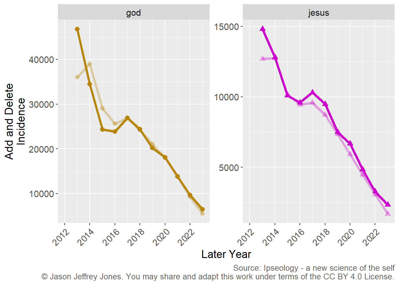
After that, we can do something very interesting: we can count the bio revision events we observe for every signifier! We’ll stick to god and jesus for now, but check Data and Code for links to data on all tokens. In Figure 5.2, compare the Add and Delete counts each year. Now we can make strong inferences about individual behavior in the aggregate.
Code
# Download a csv file containing annual events.# Read about the data in the text file at https://osf.io/57wcbtyoyl =read_csv("https://osf.io/download/gj8vt/")godJesusSignifiers =c("god", "jesus")# Visualize god and jesus Adds and Deletes over time.tyoyl %>%select("token", "lateYear", "adds", "deletes") %>%filter(token %in% godJesusSignifiers ) %>%mutate(Signifier =factor(token, levels = godJesusSignifiers) ) %>%ggplot(aes(x = lateYear, y = adds, color = Signifier, shape = Signifier)) +geom_line(linetype="solid", linewidth=1.5) +geom_point(size=2, stroke =1.25, fill ="white") +geom_line(aes(x = lateYear, y = deletes, color = Signifier), linetype="solid", linewidth=1.5, alpha =0.33 ) +geom_point(aes(x = lateYear, y = deletes, color = Signifier, shape = Signifier), size=2, stroke =1.25, fill ="white", alpha =0.33) +scale_x_continuous(limits =c(2012,2023), breaks =seq(2012,2022,2)) +#scale_y_continuous(limits=c(0,6000), breaks = seq(0,6000,1000), minor_breaks = NULL ) + scale_color_manual(values =c("god"="darkgoldenrod", "jesus"="magenta3")) +#scale_shape_manual(values = magaSignifiersShapes) +xlab("Later Year") +ylab("Add and Delete\nIncidence") +theme(text =element_text(size=14)) +theme(legend.position="none") +theme(axis.text.x =element_text(angle =45, hjust =1)) +labs(caption ="Source: Ipseology - a new science of the self\n \uA9 Jason Jeffrey Jones. You may share and adapt this work under terms of the CC BY 4.0 License.") +theme(plot.caption =element_text(size=10, color ="#666666")) +facet_wrap(vars(Signifier), scales ="free_y")
Figure 5.2: Incidence of god and jesus Add and Delete events in US bios within year-over-year longitudinal samples. Stronger lines depict Add event counts, while fainter lines depict Delete event counts. Note that the y-axes have separate scales.
In most years, the number of Add and Delete events were nearly even. There was some separation early in the god series. From 2012 to 2013, many more users added god (and jesus) than deleted. That reversed for god, however, which suffered net negative year-over-year periods in 2013-14, 2014-15, and 2015-16.
Overall, the slopes of all four series are negative. This implies that within bio revisions, god and jesus received less attention each year - with the exception of 2016-17. Think back to the decreasing prevalence of god and jesus in the cross-sectional data. We can see that it was not the result of many more users deleting rather than adding these signifiers to their bios. Instead, there must be other explanations. Perhaps newly joining and active users were less likely to include god and jesus in their bios. Perhaps those with god and jesus in their profiles left the platform or stopped tweeting as often. We don’t have to guess. Deeper investigation would reveal the paths users took.
I hope you are intrigued. I don’t know why US Twitter users added and deleted god and jesus at these rates, but we now know that they did. With the Data and Code section below, you have the resources to quickly compare god and jesus to about 20,000 other signifiers! I look forward to seeing your comparisons between signifiers of interest to you and to reading competing explanations for the trends depicted here.